Variational Integrators

Applying Lagrangian Mechanics

From Rigid Body Dynamics we learned that a mechanical system is described by generalized coordinates $\mathbf{q}$, velocities $\dot{\mathbf{q}}$, and Lagrangian $L(\mathbf{q},\dot{\mathbf{q}})=K-U$. Real motion is one that satisfies the Least Action Principle/Euler-Lagrange Equations. For rigid bodies, $\mathbf{q}$ is not just a vector in ${\mathbb{R}}^n$ but inside configuration space $\mathrm{SE}(3)$.

The theme was that mechanics is geometry (linear algebra) plus variational principles (calculus). This document takes that idea and applies it numerically to simulate physics.

Simple Numerical Methods

Standard numerical methods for solving ODEs (e.g. Forward Euler Method, or RK4) look at $F=ma$ at a specific point in time and try to blindly guess the next geometric slope. A variational integrator is a numerical method that tries to preserve the underlying geometric structure of the system. It defines the total physical energy of the system across a span of time (“discrete action”) and uses calculus to find the trajectory that minimizes this energy over time (least action paths).

In particular, we see that in this example, when $\Delta t$ is larger (i.e. $0.9$), the system is stable in “asteroid belts”. Although the system is a good approximation, as it never explodes, it is still only an approximation. We can improve the accuracy of the system by replacing the RHS of the example with

$$\frac{{\theta }_{i+1}-2{\theta }_i+{\theta }_{i-1}}{\Delta t^2}=4\arg \left(1+\frac{\Delta t^2}{4}{e}^{-i{\theta }_i}\right)$$

where $\arg$ calculates the angle of a complex number in the complex plane. The result is that the system is stable for all $\Delta t$, and removes the “asteroid belts” that we see in the previous example.

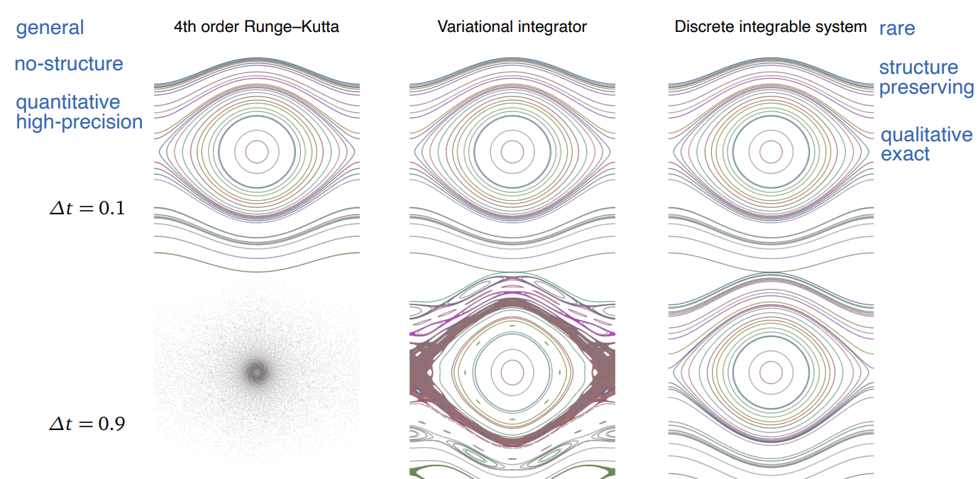
This image represents the exact trajectories on the position-momentum plane, where $\mathbf{q}$ is the $x-$axis and $\dot{\mathbf{q}}$ is the $y-$axis.

Störmer-Verlet Method

What if instead of discretizing an ODE, what if we discretize the action and take the variational derivative to get the equations of motion?

Main Idea

Standard numerical methods look at the slope of the next discretized point. A variational integrator says “among all discrete paths, which one makes the discrete action stationary?”

Let $h$ denote the discrete timestep. A discrete Lagrangian is a function

$$L_h:Q\times Q\to \mathbb{R}$$

approximating the total action between two positions. The continuous Lagrangian is Kinetic Energy minus Potential Energy:

$$L(\mathbf{q},\dot{\mathbf{q}})=\frac{m}{2}|\dot{\mathbf{q}}{|}^2-U(\mathbf{q})$$

Since we simulate this, time is broken up into steps of size $h$. The discrete Lagrangian via the trapezoidal rule (from Calculus 1!) is:

$$\begin{array}{rl}{L}_h({\mathbf{q}}_i,{\mathbf{q}}_{i+1})& =\frac{h}{2}\left(L\left({\mathbf{q}}_i,\frac{{\mathbf{q}}_{i+1}-{\mathbf{q}}_i}{h}\right)+L\left({\mathbf{q}}_{i+1},\frac{{\mathbf{q}}_{i+1}-{\mathbf{q}}_i}{h}\right)\right)\\ & =\frac{mh}{2}{\left|\frac{{\mathbf{q}}_{i+1}-{\mathbf{q}}_i}{h}\right|}^2-\frac{h}{2}\left(U({\mathbf{q}}_i)+U({\mathbf{q}}_{i+1})\right)\end{array}$$

So, the discrete total action of a path is

$$S_h({\mathbf{q}}_0,\dots ,{\mathbf{q}}_N)=\sum _{k=0}^{N-1}{L}_h({\mathbf{q}}_k,{\mathbf{q}}_{k+1})$$

or the sum of all the discrte Lagrangian segments. Remember, we want to find the minimum of these segments.

Functional

Recall that this is the total action functional seen in here but discretized (approximating a curve with $N$ small segments)!

By the discrete least action principle, $\frac{\partial S_h}{\partial {\mathbf{q}}_k}=0$ for all $k$. We can derive this similar to how we showed the LAP. Let

$$S=\sum _{k=0}^{N-1}{L}_h({\mathbf{q}}_k,{\mathbf{q}}_{k+1})$$

Then to apply LAP, we need to find a stationary point where small pertubations to the path do not change the total action. We need to find the first variation (the derivative via multivariable chain rule) denoted as $\mathring{S}$ and setting it to $0$.

$$\mathring{S}=\sum _{k=0}^{N-1}{D}_1{L}_h({\mathbf{q}}_k,{\mathbf{q}}_{k+1})\cdot {\mathring{\mathbf{q}}}_k+\sum _{k=0}^{N-1}{D}_2{L}_h({\mathbf{q}}_k,{\mathbf{q}}_{k+1})\cdot {\mathring{\mathbf{q}}}_{k+1}$$

The second term can be rewritten as

$$\sum _{k=1}^{N-1}{D}_2{L}_h({\mathbf{q}}_{k-1},{\mathbf{q}}_k)\cdot {\mathring{\mathbf{q}}}_k$$

such that

$$\mathring{S}=\sum _{k=1}^{N-1}\left(D_1{L}_h({\mathbf{q}}_k,{\mathbf{q}}_{k+1})+D_2{L}_h({\mathbf{q}}_{k-1},{\mathbf{q}}_k)\right)\cdot {\mathring{\mathbf{q}}}_k=0$$

But for this to equal $0$, the inside terms must equal $0$ exactly.

$$D_1{L}_h({\mathbf{q}}_k,{\mathbf{q}}_{k+1})+D_2{L}_h({\mathbf{q}}_{k-1},{\mathbf{q}}_k)=0$$

We can now compute the first derivative of $L_h$ with respect to ${\mathbf{q}}_k,{\mathbf{q}}_{k+1}$ gives us

$$\begin{array}{rl}{D}_{1}L{|}_{{\mathbf{q}}_k,{\mathbf{q}}_{k+1}}& =-\frac{m}{h^2}({\mathbf{q}}_{k+1}-{\mathbf{q}}_k)-\frac{dU({\mathbf{q}}_k)}{2}\\ D_{2}L{|}_{{\mathbf{q}}_{k-1},{\mathbf{q}}_k}& =\frac{m}{h^2}({\mathbf{q}}_k-{\mathbf{q}}_{k-1})-\frac{dU({\mathbf{q}}_k)}{2}\end{array}$$

implying that

$$-\frac{m}{h^2}({\mathbf{q}}_{k+1}-2{\mathbf{q}}_k+{\mathbf{q}}_{k-1})-dU({\mathbf{q}}_k)=0$$

Let

$$\mathbf{F}({\mathbf{q}}_k):=-dU({\mathbf{q}}_k)=m\frac{{\mathbf{q}}_{k+1}-2{\mathbf{q}}_k+{\mathbf{q}}_{k-1}}{h^2}$$

This is different from RK4¹

This gives us an explicitly timestep march, where $({\mathbf{q}}_{k-1},{\mathbf{q}}_k)\mapsto ({\mathbf{q}}_k,{\mathbf{q}}_{k+1})$ and so

$$\boxed{{\mathbf{q}}_{k+1}=2{\mathbf{q}}_k-{\mathbf{q}}_{k-1}+\frac{h^2}{m}\mathbf{F}({\mathbf{q}}_k)}$$

Why is this better than RK4?

The idea is that variational integrators preserve the geometric structure of the shape of motion in configuration space better than generic ODE solvers.

Stability

See prior image. The Störmer-Verlet method is the variational integrator on the right. We see a cleaner phase portrait.

Discrete Euler-Lagrange Equation

The discrete Euler-Lagrange equation is the stationarity condition for the discrete action

$$S_h({\mathbf{q}}_0,\dots ,{\mathbf{q}}_N)=\sum _{k=0}^{N-1}{L}_h({\mathbf{q}}_k,{\mathbf{q}}_{k+1}).$$

For each interior index $k=1,\dots ,N-1$, varying ${\mathbf{q}}_k$ while keeping the endpoints fixed gives

$$D_2{L}_h({\mathbf{q}}_{k-1},{\mathbf{q}}_k)+D_1{L}_h({\mathbf{q}}_k,{\mathbf{q}}_{k+1})=0$$

This is the discrete analogue of the continuous Euler-Lagrange equation. In particular, it is the general variational principle from which methods such as Störmer-Verlet Method are derived.

Interpretation

The two terms represent the two discrete action contributions meeting at the node ${\mathbf{q}}_k$: one contribution comes from the interval $[{\mathbf{q}}_{k-1},{\mathbf{q}}_k]$, and the other comes from the interval $[{\mathbf{q}}_k,{\mathbf{q}}_{k+1}]$. Their sum vanishes because the discrete path is stationary with respect to variations of the interior point ${\mathbf{q}}_k$.

This is the discrete counterpart of the continuous idea that momentum is obtained from the velocity derivative of the Lagrangian:

$$\mathbf{p}=\frac{\partial L}{\partial \dot{\mathbf{q}}}.$$

Accordingly, the discrete Lagrangian defines two discrete Legendre transforms

$$\mathbb{F}L:(\mathbf{q},\dot{\mathbf{q}})\mapsto \left(\mathbf{q},\frac{\partial L}{\partial \dot{\mathbf{q}}}(\mathbf{q},\dot{\mathbf{q}})\right)$$

by replacing the velocity description with a pair of nearby configurations. Define $f_1,f_2:Q\times Q\to T^{\ast }Q$ (the contangent bundle) by

$$\begin{array}{rl}{f}_1& :({\mathbf{q}}_1,{\mathbf{q}}_2)\mapsto \left({\mathbf{q}}_1,-D_1{L}_h({\mathbf{q}}_1,{\mathbf{q}}_2)\right)\\ f_2& :({\mathbf{q}}_1,{\mathbf{q}}_2)\mapsto \left({\mathbf{q}}_2,D_2{L}_h({\mathbf{q}}_1,{\mathbf{q}}_2)\right)\end{array}$$

The quantity

$${\mathbf{p}}_k^{-}:=-D_1{L}_h({\mathbf{q}}_k,{\mathbf{q}}_{k+1})$$

is the left discrete momentum at ${\mathbf{q}}_k$ (contribution from previous state), and

$${\mathbf{p}}_k^{+}:=D_2{L}_h({\mathbf{q}}_{k-1},{\mathbf{q}}_k)$$

is the right discrete momentum at ${\mathbf{q}}_k$ (contribution to next state). The discrete Euler-Lagrange equation is exactly the matching condition

$${\mathbf{p}}_k^{-}={\mathbf{p}}_k^{+}.$$

In terms of the maps $f_1$ and $f_2$, this says

$$f_2({\mathbf{q}}_{k-1},{\mathbf{q}}_k)=f_1({\mathbf{q}}_k,{\mathbf{q}}_{k+1}).$$

Therefore, if $f_1$ is locally invertible², we can solve for the next pair $({\mathbf{q}}_k,{\mathbf{q}}_{k+1})$ from the previous pair $({\mathbf{q}}_{k-1},{\mathbf{q}}_k)$ by applying $f_2$ and then $f_1^{-1}$. This gives the marching rule

$$({\mathbf{q}}_k,{\mathbf{q}}_{k+1})=f_1^{-1}\circ f_2({\mathbf{q}}_{k-1},{\mathbf{q}}_k)$$

Thus the discrete EL equation gives an update map on $Q\times Q$, and through the maps $f_1,f_2$ it also induces the corresponding update on phase space $T^{\ast }Q$. We can visualize this as

$"\\begin{document}\n\\begin{tikzpicture}[>=stealth, scale=1.0]\n\n$

source code

The $q\times p$ space corresponds to the axes in the image.

Variational Integrators via Midpoint Rule

The midpoint rule is a variational integrator where the discrete Lagrangian is

$$L_h({\mathbf{q}}_0,{\mathbf{q}}_1)=\underset{\text{midpoint approximation}}{\underbrace{hL\left(\frac{{\mathbf{q}}_0+{\mathbf{q}}_1}{2},\frac{{\mathbf{q}}_1-{\mathbf{q}}_0}{h}\right)}}=\frac{mh}{2}{\left|\frac{{\mathbf{q}}_1-{\mathbf{q}}_0}{h}\right|}^2-hU\left(\frac{{\mathbf{q}}_0+{\mathbf{q}}_1}{2}\right)$$

The Euler-Lagrange equation is

$$m\frac{{\mathbf{q}}_{k+1}-2{\mathbf{q}}_k+{\mathbf{q}}_{k-1}}{h^2}=\frac{1}{2}\left(\mathbf{f}\left(\frac{{\mathbf{q}}_{k-1}+{\mathbf{q}}_k}{2}\right)+\mathbf{f}\left(\frac{{\mathbf{q}}_k+{\mathbf{q}}_{k+1}}{2}\right)\right)$$

and equivalently,

$$\{\begin{array}{l}m\frac{{\mathbf{q}}_{k+1}-{\mathbf{q}}_k}{h}=\frac{{\mathbf{p}}_{k+1}+{\mathbf{p}}_k}{2}\\ \frac{{\mathbf{p}}_{k+1}-{\mathbf{p}}_k}{h}=\mathbf{f}\left(\frac{{\mathbf{q}}_{k+1}-{\mathbf{q}}_k}{h}\right)\end{array}$$

which is the implicit midpoint method. It is implicit because ${\mathbf{q}}_{k+1}$ appears on both sides, so we cannot write a simple rule for it like in Störmer-Verlet Method.

Discrete Liouville Theorem

Marching on $q\times p$ space preserves the enclosed area of the marched loop. In particular, the area is a section on the graphs we see above. This means that all possible positions and momentum are conserved as the system evolves over time.

The path the system takes between all the points may change, but the area of the path is preserved (even if the shape is complex). This geometric property is called symplecticity and is a consequence of the variational principle. This is precisely why variational integrators are better than generic ODE solvers: they preserve the underlying geometric structure of the system, which leads to better long-term stability and accuracy in simulations.

Discrete Noether’s Theorem

If the discrete Lagrangian has a continuous symmetry,

$$(\forall {\mathbf{q}}_1,{\mathbf{q}}_2\in Q)⟨D_{1}L({\mathbf{q}}_1,{\mathbf{q}}_2)\mid \mathbf{X}⟩+⟨D_{2}L({\mathbf{q}}_1,{\mathbf{q}}_2)\mid \mathbf{X}⟩=0$$

then $⟨{\mathbf{p}}_k|\mathbf{X}⟩$ is conserved (constant independent of $k$).

For example, if we let a particle move along a wire in empty space and then translate the entire system, the Lagrangian is invariant to this translation. Mathematically, let $\mathbf{v}$ be a constant vector representing the direction of symmetry, and let ${\mathbf{q}}_k$ be the start and ${\mathbf{q}}_{k+1}$ be the end of a discrete segment. The translation is by some amount $\epsilon$ along $\mathbf{v}$ is $\mathbf{q}\mapsto \mathbf{q}+\epsilon \mathbf{v}$.

$"\\usepackage{amsmath}\n\\usepackage{amssymb}\n\\usepackage{amsfonts}\n\n\\begin{document}\n\\begin{tikzpicture}[>=stealth, scale=1.3]\n\n$

source code

Because the Lagrangian is invariant to this translation, we have its derivative with respect to $\epsilon$ must be $0$.

$$\frac{d}{d\epsilon }L({\mathbf{q}}_k+\epsilon \mathbf{v},{\mathbf{q}}_{k+1}+\epsilon \mathbf{v})=0$$

By the chain rule, this is equivalent to

$$D_{1}L({\mathbf{q}}_k,{\mathbf{q}}_{k+1})\cdot \mathbf{v}+D_{2}L({\mathbf{q}}_k,{\mathbf{q}}_{k+1})\cdot \mathbf{v}=0$$

Indeed, this is true for all $\mathbf{v}$ and $k$ because of the symmetry.

We can show this is true for momentum. Recall from earlier that the discrete momentum entering the current step ${\mathbf{p}}_k$ and leaving the current step ${\mathbf{p}}_{k+1}$³ are

$$\begin{array}{rl}{\mathbf{p}}_k& =-D_{1}L({\mathbf{q}}_k,{\mathbf{q}}_{k+1})\\ {\mathbf{p}}_{k+1}& =D_{2}L({\mathbf{q}}_k,{\mathbf{q}}_{k+1})\end{array}$$

Substituting into the symmetry condition gives us

$$\begin{array}{rl}⟨-{\mathbf{p}}_k|\mathbf{v}⟩+⟨{\mathbf{p}}_{k+1}|\mathbf{v}⟩& =0\\ ⟨{\mathbf{p}}_{k+1}|\mathbf{v}⟩& =⟨{\mathbf{p}}_k|\mathbf{v}⟩\end{array}$$

Indeed, momentum along the direction of symmetry $\mathbf{v}$ is conserved across all steps $k$.

Idea

This article gives a nice intuitive explanation of Noether’s theorem and how the ideas from Lagrangian Mechanics are used to show symmetry.

Definition (Time Reversal Symmetry)

In classical physics, the equations of motion are invariant under time reversal. If our discrete integrator satisfies the property that

$$L(q_1,q_2)=-L(q_2,q_1)$$

then we say it is time-reversal symmetric. Indeed, the Störmer-Verlet Method is time-reversal symmetric.

$$\begin{array}{rlrl}{\mathbf{q}}_{k+1}& =2{\mathbf{q}}_k-{\mathbf{q}}_{k-1}+\frac{h^2}{m}\mathbf{F}({\mathbf{q}}_k)& & \text{forward}\\ {\mathbf{q}}_{k-1}& =2{\mathbf{q}}_k-{\mathbf{q}}_{k+1}+\frac{h^2}{m}\mathbf{F}({\mathbf{q}}_k)& & \text{reverse}\end{array}$$

Footnotes

1. Why? ↩

2. Here, “locally invertible” means that near a regular point, the phase-space data $({\mathbf{q}}_k,{\mathbf{p}}_k)$ uniquely determines a nearby next configuration ${\mathbf{q}}_{k+1}$. For the mechanical discrete Lagrangians used in this note, this holds whenever the discrete Lagrangian is regular, which is typically true for sufficiently small timestep $h$. ↩

3. The negative sign is from the original Discrete Euler-Lagrange equation as described previously. ↩