Vorticity

Definition (Vorticity Field)

A vorticity field is a continous distribution of of vorticity throughout the entire fluid domain. Because velocity varies from point to point in a fluid, the curl varies from point to point. Indeed, it defined as

$$\mathbf{w}:=\nabla \times \mathbf{u}=\text{curl }\mathbf{u}$$

In 2D, this is a scalar field, while in 3D, this is a vector field.

Imagine we placed a small paddle wheel in the fluid. If the wheel spins, then there is vorticity at that point. In 3D, the vorticity field must be divergence-free. By Stokes Theorem, the circulation along some boundary $C$ is the integral of the vorticity over $\Sigma$.

$${\Gamma }_C={\oint }_C\mathbf{u}\cdot d\ell ={\iint }_{\Sigma }\mathbf{w}\cdot \mathbf{n}dA$$

By Kelvin’s Circulation Theorem, the flux of vorticity across a surface flowing with fluid is constant in time.

Definition (Vortex Line)

A vortex line is a curve tangential to the vorticity field.

• We will see that a vorticity field can be viewed as infinitely many threads of infinitesimal vortex lines (these are the “atoms”).
• The integral of vorticity through a surface is how many vortex lines pass through the surface.
• Vorticity magnitude is the cross-sectional density of vortex lines. The more vortex lines per unit area, the stronger the vorticity.
• Vortex lines are passively advected by the flow. This means wrt a fluid particle, the vortex lines move with the particle.

$"\\usepackage{tikz}\n\\usetikzlibrary{decorations.markings}\n\n\\begin{document}\n\\begin{tikzpicture}\n\n$

source code

We can think of vortex lines as picking some arbitrary point in the fluid, and tracing out the curve that is always tangential to the vorticity field, by following the direction of the vorticity vector at each point. Tracing these points for infinitely many points gives us our curve.

Preservation of Vortex Lines / Helmholtz’s Theorem

If a curve or surface is tangential to the vorticity field, and flows with the fluid, then the curve or surface remains tangential to the vorticity field over time.

Intuition & Proof:

• The Surface Case: Being tangential to the vorticity field means no vortex lines cross or pierce the surface. Mathematically, this means the vorticity flux across the surface is exactly zero.
• The Conservation: By Kelvin’s Circulation Theorem, the vorticity flux across any material surface is constant over time. Since the flux starts at zero, it must remain zero forever. Therefore, the surface never crosses a vortex line and remains permanently tangential.
• The Curve Case: A single 1D vortex line (curve) can be defined locally as the geometric intersection of two 2D tangential surfaces. Because both surfaces perfectly follow the fluid motion without crossing vortex lines, their intersection is permanently glued to the fluid particles.

Definition (Vortex Tube)

A vortex tube is taking a surface $S$ nowhere tangent to the vorticity field, and collecting all vortex lines extending from $S$.

Idea

If a single vortex line is a thread, then a vortex tube is a bundle of threads (or a solid cable). We are essentially tracing infinitely many tubes.

Also they really do look like tubes.

Theorem (Circulation is Constant)

If $C_1,C_2$ are two closed curves encircling the tube, then ${\Gamma }_{C_1}={\Gamma }_{C_2}$. In other words, the circulation around any closed curve encircling the tube is the same.

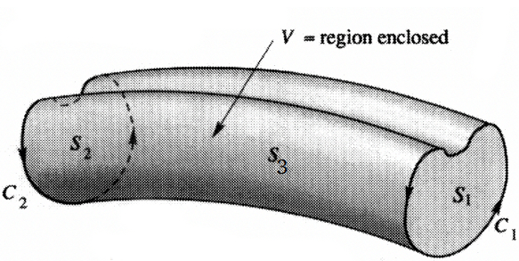
Proof: Apply Divergence Theorem on vorticity field in $V$, the region enclosed. Note that vorticity has no divergence, so $\nabla \cdot \mathbf{w}=0$.

$$\begin{array}{rl}{\iiint }_V\nabla \cdot \mathbf{w}dV& ={\iint }_{\partial V}\mathbf{w}\cdot \mathbf{n}dA\\ 0& ={\iint }_{S_1}\mathbf{w}\cdot \mathbf{n}dA-{\iint }_{S_2}\mathbf{w}\cdot \mathbf{n}dA+{\iint }_{S_3}\mathbf{w}\cdot \mathbf{n}dA\\ 0& ={\iint }_{S_1}\mathbf{w}\cdot \mathbf{n}dA-{\iint }_{S_2}\mathbf{w}\cdot \mathbf{n}dA+0\\ 0& =0\end{array}$$

In $S_3$, the walls of the tube are tangential to the vorticity field, so no vortex lines cross $S_3$. Therefore, the flux of vorticity across $S_3$ is zero. The flux across $S_1$ and $S_2$ must be conserved, so they are equal.

Definition (Strength of a Vortex Tube)

Call this circulation the strength of the vortex tube.

Theorem (Vortex Strength is Constant)

As the vortex tube is flowing with the fluid, the vortex strength is constant over time.

Vortex Branches

In case the tube branches, the strength of from each branch adds up since vorticity cannot be created or destroyed out of nowhere (divergence-free). The circulation of the main trunk will always equal to the sum of the circulations of its branches.

$"\\usepackage{tikz}\n\\usetikzlibrary{decorations.markings}\n\n\\begin{document}\n\\begin{tikzpicture}\n\n$

source code

Smoke rings (closed-loop vortex tubes) are a common example of vortex tubes. They are stable because an isolated vortex tube cannot just end; it must either

• form a closed loop
• extend to the boundaries of the fluid domain
• branch infinitely

Definition (Vortex Filaments/Sheets)

Vortex filaments are concentrated vortex tubes. It is the limit of a vortex tube as its cross-sectional area shrinks to zero with finite strength. We can think of it as squeezing vortex tubes until they become infinitely thin (1D curves) while keeping the strength constant.

Vortex Sheets are vortex tubes that are squished completely flat into a 2D surface. It represents a severe, discontinuous jump in the fluid’s velocity field. For example, if we have wind blowing the opposite direction over another gust of wind, the boundary between the two layers of air is a vortex sheet.

Vorticity Equation

In 3D, the vorticity field is transported by the flow

$${\mathbf{w}}_t={\mathbf{F}}_t{\mathbf{w}}_0\text{where }{\mathbf{F}}_t=d{\varphi }_t$$

One can show that

$$\underset{\text{advection}}{\underbrace{\frac{\partial }{\partial t}\mathbf{w}+{\nabla }_{\mathbf{u}}\mathbf{w}}}=\underset{\begin{array}{c}\text{vortex}\\ \text{stretching}\end{array}}{\underbrace{{\nabla }_{\mathbf{w}}\cdot \mathbf{u}}}$$

The physical interpretation of the left side is that vorticity is being advected by the flow (carried by the flow)¹. The right side is the vortex stretching term, which is unique to 3D. It represents how the vorticity can be amplified by the flow.

For example, imagine we have a thick vortex tube spinning in the fluid

Going back to the literal water vortex analogy, we have a many vortex lines bundled together in a tube.

What happens when the velocity field of the fluid pulls the top and bottom of that tube, stretching it out?

The literal vortex will grow because the movement of water is increasing the literal vortex size.

Because the fluid is incompressible, the cross-sectional area of the tube must shrink to keep the same strength, by Theorem (Vortex Strength is Constant). By conservation of angular momentum, the tube must spin faster to compensate for the smaller cross-sectional area.

Like an ice skater pulling in their arms to spin faster, the vortex tube must spin faster to maintain the same strength.

This deformation of the tube is expressed mathematically with ${\mathbf{F}}_t$ (note the time $t$). It shows how a tiny, perfect cube of fluid gets squished, stretched, and tilted as it flows through space over time.

2D Case

In 2D, the vorticity field is a scalar function transported by the flow:

$$\frac{\partial }{\partial t}w+{\nabla }_{\mathbf{u}}w=0$$

Reconstructing Velocity from Vorticity

If we decide to simulate a fluid by tracking its vorticity instead of its velocity, we encounter an obvious problem: we still need the velocity to actually move the fluid particles.

Biot-Savart Law

In electromagnetism, the Biot-Savart law states that a wire carrying an electric current produces a magnetic field. In fluid dynamics, the Biot-Savart law states that a vortex tube produces a velocity field.

Biot-Savart Integral

Let $\mathbf{w}$ be the vorticity field in the fluid. If the fluid domain is the entire ${\mathbb{R}}^3$, then there is a unique divergence-free velocity field $\mathbf{u}$ which decays to zero at infinity.

$$\mathbf{u}(\mathbf{x})=\frac{1}{4\pi }{\int }_{\text{supp}(\mathbf{w})}\frac{\mathbf{w}(\mathbf{y})\times (\mathbf{x}-\mathbf{y})}{|\mathbf{x}-\mathbf{y}{|}^3}dV(\mathbf{y})$$

where

• $\mathbf{u}(\mathbf{x})$ is the velocity at point $\mathbf{x}$ in the fluid
• $\mathbf{w}(\mathbf{y})$ is the vorticity at point $\mathbf{y}$ in the fluid
• The cross product $\times$ guarantees that the velocity field is always perpendicular to the vorticity field.
• The denominator $|\mathbf{x}-\mathbf{y}{|}^3$ ensures that the influence of vorticity at $\mathbf{y}$ on the velocity at $\mathbf{x}$ decays with distance, following the Inverse Square Law in 3D.
• The $\text{supp}(\mathbf{w})$ is the Support of the vorticity function $\mathbf{w}$, the set of points in the domain where the function’s value is not zero. It is the points in our domain where the fluid is actually swirling.

For 2D, the Biot-Savart law is

$$\mathbf{u}(\mathbf{x})=\frac{1}{2\pi }{\int }_{\text{supp}(w)}\frac{w(\mathbf{y})R^{90^{\circ }}\times (\mathbf{x}-\mathbf{y})}{|\mathbf{x}-\mathbf{y}{|}^2}d{A}_{\mathbf{y}}$$

where $R^{90^{\circ }}$ is the 90 degree rotation matrix and $\text{supp}(\mathbf{w})$.

When vorticity is concentrated into codimension-2² geometry (vortex filament in 3D or point vortex in 2D), the Biot-Savart law simplifies significantly.

First, since the filament must be closed, with a fixed strength

$$\kappa ={\oint }_{\begin{array}{c}\text{any loop}\\ \text{around }\Gamma \end{array}}{\mathbf{u}}^{♭}$$

such that

$$\mathbf{u}(\mathbf{x})=\frac{\kappa }{4\pi }{\int }_{\Gamma }\frac{T(\mathbf{y})\times (\mathbf{x}-\mathbf{y})}{|\mathbf{x}-\mathbf{y}{|}^3}d{s}_{\mathbf{y}}$$

where

• $\Gamma$ is the curve representing the vortex filament,
• $T(\mathbf{y})$ is the unit tangent vector. Because the filament is infinitely thin, the complex 3D vorticity vector $\mathbf{w}$ is perfectly replaced by just the direction the curve is pointing $\mathbf{T}$ multiplied by the strength $\kappa$,
• $d{s}_{\mathbf{y}}$ is the line element along the curve $\Gamma$, which accounts for the length of the curve segment at $\mathbf{y}$.

Idea

We now no longer need to simulate the fluid as a 3D field. Instead, we can just track the 1D curve of the vortex filament and its strength. This is a huge simplification that allows us to simulate fluids with less computational resources.

In 2D,

$$\mathbf{u}(\mathbf{x})=\sum _i\frac{{\kappa }_i}{2\pi }\frac{R^{90^{\circ }}(\mathbf{x}-{\mathbf{y}}_i)}{|\mathbf{x}-{\mathbf{y}}_i{|}^2}$$

Because a 0D point has no length, we only need to sum over the discrete set of point vortices.

Biot-Savart Integral: Obstacle Treatment

The fatal flaw of the Biot-Savart integral is that it only works for infinite domains. It assumes the domain is infinitely large and completely empty. An obstacle (like a rock in a river) will calculate the velocity field that flows through the rock, which is (obviously) physically impossible.

Therefore we must modify the Biot-Savart field with a gradient field (i.e. a pressure projection).

• Solve the Laplace problen in the outer domain with Neumann boundary condition
• Classically done with boundary element method
• Or by Kelvin Transformation.

Stream Function

Instead of an $O(n^2)$ Biot-Savart integral, we can solve the PDE to find the velocity. Consider the followingn ansatz:

$$\begin{array}{rlrl}\mathbf{u}& =\nabla \times \Psi & & \text{in 3D}\\ \mathbf{u}& =-R^{90^{\circ }}\nabla \psi & & \text{in 2D}\end{array}$$

where $\Psi$ is the vector potential in 3D and $\psi$ is the scalar stream function in 2D. The first equation ensures the incompressibility condition $\nabla \cdot \mathbf{u}=0$ is automatically satisfied. We can plug this ansatz into the definition of vorticity $\mathbf{w}=\nabla \times \mathbf{u}$ to get

$$\nabla \times (\nabla \times \Psi )=\mathbf{w}$$

and get (not sure how to derive this)

$$-\Delta \Psi =\mathbf{w}$$

In 2D, this is just $-\Delta \psi =w$ with $\psi =0$ on the boundary.

Beware the result could be incorrect if there are multiple boundary components, or that the domain is non-simply-connected.

Paper

Helmholtz-Hodge-Morrey-Friedrichs

In general, we have the following orthogonal decomposition

$$\begin{array}{rlrl}\tilde{\mathbf{u}}& =\nabla p+\nabla \times \Psi +\mathbf{h}& & \text{in 3D}\\ \tilde{\mathbf{u}}& =\nabla p-R^{90^{\circ }}\nabla \psi +\mathbf{h}& & \text{in 2D}\end{array}$$

with $\Psi$ normal to the boundary and $\psi$ zero on the boundary.

$$\{\begin{array}{ll}\nabla \cdot \mathbf{h}=0& \\ \nabla \times \mathbf{h}=0& \\ \mathbf{h}\cdot \mathbf{n}=0& \text{on the boundary}\end{array}$$

Vortex Methods

We want to discretize the fluid by tracking its vorticity instead of its velocity. This is called the vortex particle method. In 3D, vorticity is done by measuring its vortex filaments

$$\underset{\text{vec}}{\underbrace{{\varphi }_t^{\ast }}}{\mathbf{w}}_t={\mathbf{w}}_0$$

and in 2D its point vortices

$$w_t\circ {\varphi }_t=w_0$$

The vortex particle method makes little sense in 3D, because the vorticity must be divergence free, all vortex lines must form a closed loop or extend infinitely to the boundaries of our fluid domain. Otherwise, we have fluid flowing from one place to another and stopping (creating a sink)³.

2D Vortex Particle Algorithm

We can turn the problem into a discrete $N-$body physics problem. Instead of a fluid, imagine we have a handful of active particles.

Each particle has a fixed vorticity strength ${\kappa }_p$ which can be positive or negative. The 2D position of each particle ${\varphi }_p$ is described by

$$\frac{d}{dt}{\varphi }_p=\sum _{\begin{array}{c}q\in \text{VortexParticles}\\ q\ne p\end{array}}\frac{{\kappa }_q}{2\pi }\frac{R^{90^{\circ }}({\varphi }_p-{\varphi }_q)}{|{\varphi }_p-{\varphi }_q{|}^2}$$

Then, we evaluate velocity for any passively advected smoke/dye by

$${\mathbf{v}}_{\mathbf{x}}=\sum _{\begin{array}{c}q\in \text{VortexParticles}\end{array}}\frac{{\kappa }_q}{2\pi }\frac{R^{90^{\circ }}(\mathbf{x}-{\varphi }_q)}{|\mathbf{x}-{\varphi }_q{|}^2}$$

then solve the ODE by RK4.

3D Vortex Filament Algorithm

This is extremely hard. Filaments stretch, twist, grow exponentially, need reconnection…

Recall the continuous PDE for 3D vorticity:

$$\frac{\partial }{\partial t}\mathbf{w}+{\nabla }_{\mathbf{u}}\mathbf{w}={\nabla }_{\mathbf{w}}\mathbf{u}$$

Most papers solve this by splittng advection and stretching into two separate steps. This is unstable since the stretching step is calculated as an explicit addition, causing errors to accumulate. A better approach is to “do a semi-Lagrangian pullback for 2-form”.

The original velocity-based semi-Lagrangian approaches $\dot{\mathbf{u}}+{\nabla }_{\mathbf{u}}\mathbf{u}=0$ typically did

$${\mathbf{u}}_{t+\Delta t}(bx)={\mathbf{u}}_t({\psi }_{\Delta t}(\mathbf{x}))$$

where ${\psi }_{\Delta x}(\mathbf{x})=\mathbf{x}-\Delta t{\mathbf{u}}_t(\mathbf{x})$ is the traceback to find the old velocity at the past location ${\mathbf{u}}_t$. This ignores deformation.

Instead, we need to change what velocity physically represents. Instead of it being a vector ($0-$form), it needs to be a covector ($1-$form), a measurement of flow along a line segment. That way, if the fluid deforms at some segment, the velocity measurement scale to conserve energy.

$$\dot{\mathbf{u}}+{\nabla }_{\mathbf{u}}\mathbf{u}=-(\nabla \mathbf{u}{)}^{\top }\mathbf{u}$$

Then, we can do a semi-Lagrangian pullback for 1-form:

$${\mathbf{u}}_{t+\Delta t}(bx)=(d{\psi }_{\Delta t}{)}^{\top }({\psi }_{\Delta t}(\mathbf{x}))$$

Then velocity is transported as a covector. In particular, the Kelvin’s Circulation Theorem holds.

Additional Conservation Laws

There are more invariants of the flow besides circulation.

Theorem (Generalized Kelvin’s Circulation Theorem)

We can generalize Theorem (Kelvin’s Circulation Theorem). If $\mathbf{u}$ is a velocity field and $\mathbf{v}$ is any divergence-free vector field transported by the fluid, then

$$\int ⟨\mathbf{u},\mathbf{v}⟩dV$$

is constant.

Definition (Helicity)

$$\mathcal{H}:=\int ⟨\mathbf{u},\mathbf{v}⟩dV$$

Theorem (Helicity is Constant)

Helicity is a constant of time.

Theorem (Vortex Line Area Conservation)

In fluids, the total area of vortex lines is conserved. Vortex lines are twisted and bent curves. In ${\mathbb{R}}^3$, if we project them onto the $xz,yz,xy$ planes, we describe the area vector, $A=[A_{xz},A_{yz},A_{xy}{]}^{\top }$. The total area vector of all vortex lines is conserved.

Airplane Example

This theorem explains why airplanes can fly.

Footnotes

1. Think of a literal water vortex in a fast moving river being carried downstream. ↩

2. In a 3D fluid simulation, codimension-2 means the vortex filament is a 1D curve ($3-1=2$). In a 2D fluid simulation, codimension-2 means the point vortex is a 0D point ($2-0=2$). ↩

3. Apparently this is like the magnetic monopole problem in electromagnetism. ↩